간단 설명

1. 다른 강화학습 기법(Q-learning, Sarsa 등..)과 달리 Next state가 없고 오직 Action, Reward 의 형태를 다룬다.

2. Markov Decision Process(MDP) 환경에서 동작시키는 것이 아니다.

3. MAB는 Exploration을 어떻게 할 것인지에 대해 다양한 방법을 제시했다.


용어 설명

1. Regret

- v_*는 현재 state에서 얻을 수 있는 최대 보상값이다.

- v는 현재 state에서 MAB Agent가 action 함으로써 얻는 보상값이다.

- 현재 상태에서 수행한 action에 대한 평가값이라 생각한다.


2. Total regret

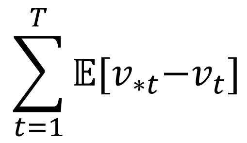
- 왼쪽의 Summation 은 시작지점(Start) t = 1 에서 끝지점(Terminal) T 까지 모두 더한다는 의미이다.

- E[v_*t - v_t]는 t 시점에서 얻었던 Regret 값에 대한 기대값이다. 기대값인 이유는 MAB를 적용할 실제 환경은 확률적이라 가정하기 때문이다.

- 시작지점 -> 끝지점 까지의 Expected Regret값을 Total regret 이라한다. MAB Agent는 이 값을 낮추기 위해서 학습한다. 

Total regret을 낮춘다는 것은 Total reward (Return)을 높인다는 것과 같다.


3. Q - function 

- MAB 프레임워크에서는 단순하게 action a를 했을때 즉각적으로 얻을 수 있는 expected reward 값이다. expected 가 있는 이유는 확률적인 환경에서 MAB를 구동시키기 때문이다.


Exploration 전략

1. Epsilon-greedy strategy

요약 설명

- epsilon 이라는 Threshold 값을 두고 확률적으로 Random 선택을 하는 방법이다.

- episode가 끝날때 마다 epsilon 값을 지정한 decay_value 만큼 감소 시킨다.

- 많은 episode가 지나면 epsilon 값이 0에 수렴하게 되는데 이때부터는 greedy 하게 선택한다.

내 생각

- 이 방법은 강화학습 프레임워크에서 많이 쓰인다. 최근에 논문을 구현하면서 사용했다.(DQN, SAC, DDPG 등등)

start episode
...
    if np.random.uniform() > epsilon:
        action = np.argmax(Q)
    else:
        action = np.random.randint(len(Q))
    
    reward = env.step(action)
    N[action] += 1
    Q[action] = Q[action] + (reward - Q[action])/N[action]
...
end episode

epsilon -= decay_value

2. Optimistic intialization strategy

요약 설명

- Q 값을 높게 잡고 greedy 하게 여러 episode를 거친다. 여기서 높게라는 의미는 기대하는 expected reward 값보다 높게 잡는 것이다.

- 여러 episode를 거치면서 자동으로 Q값들이 낮아지며 결국 모든 action에 대해 expected reward 값을 알게될 것이다.


내 생각

- epsilon-greedy 처럼 if 분기점이 필요없어서 깔끔한 코드가 될 것 같다. 

- 단점은 MAB 뿐만아니라 강화학습의 고질적인 문제는 너무 많은 Sampling을 해야한다는 것이다.

Q = np.full(env.action_space.n, optimistic_estimate)
N = np.full(env.action_space.n, initical_count)

...
#only
action = np.argmax(Q)
reward = env.step(action)
N[action] += 1
Q[action] = Q[action] + (reward - Q[action])/N[action]

3. Softmax strategy 

요약 설명

- B 는 action space 집합이다.

- tao 값은 episode가 끝날때마다 감소한다.

- tao 값이 크면 Softmax 의 확률 분포가 균등하게 나타난다. tao 값이 작으면 Q-function의 값에 따른 확률 분포가 나온다.

- 결국 처음에는 exploration, 후반에는 greedy 하게 선택하는 원리이다. 

- 딥러닝 Output fuction 계열에서 확률 분포로 쓰이는 Softmax와 똑같은 원리로 쓰인다.

scaled_Q = Q / tao
norm_Q = scaled_Q - np.max(scaled_Q)
exp_Q = np.exp(norm_Q)
probs = exp_Q / np.sum(exp_Q)

action = np.random.choice(np.arange(len(probs)), size=1, p=probs)[0]

reward = env.step(action)

tao -= decay_unit

4. Upper confidence bound(UCB) strategy

요약 설명

- Q값의 추정치가 불확실한 경우 해당 Q 값을 exploration 할 수 있도록 장려하는 방법이다.

- argmax 대괄호 안에 오른쪽 텀을 U_t 라 함.

- U_t 의 e 는 현재까지 모든 action을 한 횟수, N_e(a) 는 현재까지 action a를 수행한 횟수.

- 모든 action 대비 현재 action a를 적게할 경우 U_t 값이 증가한다. 

- 같은 action을 많이 할 경우 U_t 텀이 작아진다.

- c는 U_t 텀에 대한 가중치 이다.

U_t = np.sqrt(c * np.log(e)/N)
action = np.argmax(Q + U_t)

reward = env.step(action)

5. Thompsom sampling strategy

요약 설명

- Q 값이 가우시안 분포를 따르는 것으로 시작한다. (평균, 표준편차)

- Agent가 계속 action을 수행 할 수록 평균값은 명확해지고 표준편차는 줄어든다.

- alpha, beta 파라미터를 이용한다.

- alpha와 beta는 action space의 사이즈만큼 존재한다.

- alpha는 Q값의 초기 표준편차 값을 의미한다. alpha는 episode를 반복할수록 줄어드는데 beta는 alhpa값이 감소하는 속도를 조절한다.

samples = np.random.normal(loc=Q, scale=alpha/(np.sqrt(N) + beta))
action = np.argmax(samples)

reward = env.step(action)

written by dongheeh, hyejinp

1. Machine Learning Workspace Introduction

“All-in-one web-based development environment for machine learning”
This tool provides a docker image with an already built machine learning workspace. One of the advantages of this is web-based. Linux desktop GUI can access through a web browser. Using ml-workspace, it gives convenience to machine learning model development.


 Here is the ml-workshop github: https://github.com/ml-tooling/ml-workspace 
 

There are lots of ultimate tools for developers. Among them, we ran Jupyter Notebook which is web-based IDEs for data processing and Netdata for monitoring hardware status. We also verified by using pre-installed machine learning libraries such as pytorch, sklearn, pandas in the process.
 We are working on a movie recommendation model system project, so we tried to preprocess this model and data using this tool.


GitHub - ml-tooling/ml-workspace: 🛠 All-in-one web-based IDE specialized for machine learning and data science.

🛠 All-in-one web-based IDE specialized for machine learning and data science. - GitHub - ml-tooling/ml-workspace: 🛠 All-in-one web-based IDE specialized for machine learning and data science.

github.com


2. How to install

First, install the WSL2

1. In Windows Powershell

Executes a shell command in Windows Powershell.

Enable-WindowsOptionalFeature -Online -FeatureName Microsoft-Windows-Subsystem-Linux

2. In Microsoft Store

Install the Ubuntu 20.04.4 LTS

3. Reboot your computer

Second, install and setup the docker

1. here the download link and click the Docker Desktop for Windows

https://docs.docker.com/get-docker/


Get Docker


docs.docker.com

2. Reboot your computer


What is docker?

Docker is an open source project that runs and manages Linux applications as containers using process isolation technologies. Here's a quote from the Docker web page:


A Docker container wraps some kind of software in a complete filesystem that contains everything needed to run the software. This includes code, runtime, system tools, system libraries, anything that is installed on the server. This guarantees that it will always run the same regardless of the environment in which it is running.

https://en.wikipedia.org/wiki/Docker_(software)


Docker (software) - Wikipedia

From Wikipedia, the free encyclopedia Jump to navigation Jump to search Software for deploying containerized applications This article is about the OS-level virtualization software. For the company, see Docker, Inc. Docker is a set of platform as a service

en.wikipedia.org


Third, Getting Started Machine Learning Workspace 


1. Executes a shell command in cmd.

docker run -p 8080:8080 mltooling/ml-workspace:0.13.2

and then it will download many files.

 you will see this cmd state(don't close the cmd)

2. Open new explore or chrome etc.. and go this link (http://localhost:8080)

and you will see Web-based Jupyter Notebook 

3. Desktop GUI (Optional)

Open Tool -> VNC Click!


As the language setting of my browser is Korean, it is indicated as a "연결" button in the image below.
Click this button.

and then you will see below image

Enjoy!!


Apply to My movie recommendation system

1. Use Jupyter Notebook to data preprocessing

What is Jupyter Notebook?

Jupyter notebook is the one of web-based IDEs that allows you to run Python step by step. It can create and share documents containing live code, equations, visualizations, and narrative text and used for data cleaning and transformation, numerical simulation, statistical modeling, data visualization, machine learning, and more. In our project, data preprocessing is required to collect user responses. We can check this conveniently in Jupyter Notebook.


https://en.wikipedia.org/wiki/Project_Jupyter


Project Jupyter - Wikipedia

From Wikipedia, the free encyclopedia Jump to navigation Jump to search Nonprofit organization developing open-source software Project JupyterAbbreviationJupyterFormationFebruary 2015; 7 years ago (2015-02)Typenonprofit organizationPurposeTo support int

en.wikipedia.org


First.  Write code for data preprocess and Data upload

Second. Execute code on jupyter

2. Check my hardware state by using Netdata(optional)

What is Netdata?

Netdata is a real-time monitoring program to Linux, and the amount of hardware usage such as RAM of the computer currently in use is arranged in a table. We can easily check the figures in real-time every moment at a glance. After running the model, it allowed us to check our hardware status.

https://en.wikipedia.org/wiki/Netdata


Comment

It comes with the basic modules necessary to carry out a machine learning project, which is very convenient when starting a project. In addition, since it operates based on Docker, projects can be carried out regardless of a specific environment, so even novice programmers can easily build a machine learning environment. It helps.

However, from the point of view of an experienced programmer, it is not necessary. It accommodates more modules than expected, but because it is a workspace, memory can be wasted.
In addition, if a real-time streaming service is required to be applied to our movie recommendation project, it is better to run it in the host rather than serving it in the ML workspace.

시스템 설계

STATE

자료구조 :  Dictionary

key : snr1, snr2, snr3, snr4 -> 정수형 으로 변환후 저장.

value : Action value function (2개씩 고르는 모든 경우의 수를 가짐)


이유 :

Dictionary쓰는 이유 4개의 vector를 좀 더 단순하게 다루기 위해 문자열로 변환 후 저장 하면 그 값 자체가 고유의 key를 의미 하기 때문. (ex:  key : '10,2,3,-1', value : [10,2,0,2,1,3] ).

REWARD

첫번째 시도 -> 특정 값에 수렴하지만 최적의 값은 아니 었음.

Reward : 차분값을 이용한 방법

(select SNR 적용 후 처리율 - 이전 처리율) + (선택)(select SNR 적용 후 fairness - 이전  fairness)


두번째 시도 -> 기존의 MR Scheduling과 동일한 성능.

Reward : 해당 상태에서 뽑아냈던 최대 처리율과 현재 선택한 snr의 최대 처리율의 차분값을 이용

선택한 SNR이 이전에 선택했던 최대 처리율 보다 높으면 positive 값 적용

선택한 SNR이 이전에 선택했던 최대 처리율 보다 낮으면 negative 값 적용

(select SNR 적용 후 처리율 - 이전 최대 처리율) + (선택)(select SNR 적용 후 fairness - 이전  fairness)


이유 : 목적이 처리율이므로.  선택적으로 fairness를 고려할 수도 있음.

ACTION

epsilon-greedy (1 iteration : epsilon /= 1.5)

P(epsilon) -> greedy

P(1-epsilon) -> random


이유 : 잘못된 초기화 값을 대비하여 구성

UPDATE

Q(s,a) = Q(s,a) + alpha * (Reward + gamma * argmax(Q(s',a)) - Q(s,a))


Q-Learning 기반 ->

빠른 convergence 결과를 볼 수 있음 + 상대적으로 많이 쓰임.


학습 및 시뮬레이션 그래프


Time domain

시간에 따라 변하거나 불변하거나 하는 데이터를 다루는 차원을 의미합니다.

예시를 들어 보자면

 - 초 단위로 움직이는 시계의 초침의 회전 각도, 또는 시계 원점 기준으로 변하는 초침 끝의 X, Y 좌표


 - 설정 fps 마다 다른 단위의 시간으로 바뀌는 영상 


 - 음악을 들을 때 박자 단위로 바뀌는 음


 일상생활에 흔하게 볼 수 있는 것들입니다.

위의 예시 중 시계 예시를 들어 보겠습니다. 

시계를 이용한 Time domain 예시 1 

X축 : 초 단위

Y축 : 초침 끝 X축의 위치

측정 시작 시각 : 00시 00분 00초

시계의 반지름 :  5(단위 생략) 


x : 초, y : 초침의 x축 위치


코드 구현을 어느 정도 해보신 분들은 다시 겠지만 X 축이라 cos 그래프를 예상했을 수도 있습니다.

설명에서 시계는 00시 00분 00초 즉 90도부터 시작하기 때문에 phase shift로 인해 sin 그래프로 보입니다.

import math 
import matplotlib.pyplot as plt
import numpy as np
#반지름이 5인 시계
watchsize = 5

#초침의 시작점은 00시00분00초 시작점
#degree는 90도
startRadian = math.pi / 2 

x = np.linspace(-2, 0, 2000)
time = np.linspace(60, 0, 2000)
y = []

for addRadian in x:
    y.append(watchsize * math.cos((math.pi * addRadian) + startRadian))

plt.xlabel('second')
plt.ylabel('second hand x location')
plt.plot(time,y, )

위의 코드를 실행시키려면 아나콘다 환경에서 numpy, matplotlib를 설치해야 확인할 수 있습니다.

Time domain으로 데이터를 표현하면 이처럼 시간에 따라 변하는 데이터를 좀 더 직관적으로 표현할 수 있습니다.

하지만 이런 Time domain의 데이터를 모두 담기에는 너무 많은 용량이 필요하게 될 것입니다. 왜냐하면 시간은 흐르고(X축 증가), 시계는 고장 나지 않는 이상 초침의 X축 위치는 계속 변하기(Y축 변동) 때문입니다. 그리고 Time domain에서의 상세한 분석은 어느정도 한계가 있습니다. 이 부분은 무선 통신 분야로 설명하겠습니다.


무선채널에서의 신호를 이용한 Time domain 예시 2 

무선 채널 환경에서는 노이즈가 존재합니다. 이 노이즈가 섞인 수신 데이터들은 Time domain으로 해석한다면 원하는 신호와는 거이 다른 신호가 되어있겠죠.

Band-Pass filter 적용전 cos 송신 신호 

Band-Pass filter는 실제 무선채널 환경에 내보내기 전에 신호에 적용하는 필터입니다. 현 포스팅에서는 다루지 않겠습니다.  위의 신호를 수신단에서 수신하면 어떻게 되어 있을까요?

위의 cos 송신 신호를 수신했을때 신호


import math 
import matplotlib.pyplot as plt
import numpy as np
import random 

#-0.5~0.5 사이의 랜덤 값 추출
def makeNoise():
    if (random.random()>0.5):
        return random.random() / 2
    else:
        return -random.random() / 2

#증폭 1
amplitude = 1

#위상차이 0
phaseshift =0


x = np.linspace(0, 0.5, 200)
y = []

for addRadian in x:
    y.append((amplitude * math.cos((math.pi * addRadian) + phaseshift)) + makeNoise())
    #y.append((amplitude * math.cos((math.pi * addRadian) + phaseshift)))

plt.plot(x,y)

노이즈 채널은 상용하고 있는 채널 모델은 아닙니다. 간단하게 -0.5~0.5 사이의 값만 랜덤으로 적용시킨 것입니다. 

채널 모델 부분도 현 포스팅에서는 다루지 않겠습니다. 


이처럼 노이즈 포함된 신호가 되어있을 것 입니다. 이럴 경우 Time domain으로의 수신 신호 분석은 힘들어질 것 입니다.

하지만 이 신호를 Frequency domain으로 분석한다면 좀 더 해석하기 용이하게 변합니다. 


Time domain의 설명은 여기까지 입니다. 몇 가지 내용이 더 있지만, 이번 포스팅의 목표는 Time domain과 Frequency domain을 duality 측면에서 인사이트를 얻는 것 이기 때문입니다. 


공부중에 매트랩의 sinc 함수를 찾지 못해서

매트랩은 아니지만 python 전용으로 sinc 함수를 만들어 봤다. 주의할 부분은 sin 함수 안의 매개변수 값의 단위가 degree 인지 radian 인지 명확히 인지 해야 한다. python math의 sin은 radian이다.

즉  3.141592 radian = 180 degree이다.


sinc 함수 표현 식, https://kr.mathworks.com/


Code
import math 
import matplotlib.pyplot as plt
import numpy as np

def sinc(x):
    if x == 0:
        return 1
    else:
        return (math.sin(math.pi * x) / (math.pi * x))

x = np.linspace(-5,5,1000)
y = []

for valueX in x:
    y.append(sinc(valueX))


plt.plot(x,y)
plt.show()
결과


첫 줄 입력 자연수 N(3 <=N <=100), 자연수 K (1 <=K <=50)

둘 째줄 입력 자연수 1 ~ 100 사이의 자연수 N개의 배열


N개의 배열에서 3개의 값을 조합하여 구할 수 있는 값 중에 K 번째로 큰 값 구하기

주의해야 할 처리 사항 : 중복 숫자 값 입력 가능, K 번째 큰 수에서 중복하는 값은 무시 (ex. [5,5,4,2]에서 2번째로 큰 값은 4)

def find(arraySortedData, index, arraySumData, arrayMaxData,depth):
        
    if depth == 3:
        arrayMaxData.append(arraySumData[0])
        return
    
    for i in range(index, len(arraySortedData)):
        arraySumData[0] += arraySortedData[i]
        find(arraySortedData, i + 1, arraySumData, arrayMaxData, depth + 1)
        arraySumData[0] -= arraySortedData[i]
    

N, K = map(int, input().split())
arrayData = list(map(int,input().split()))
arrayMaxData = []
arraySumData = [0]

find(arrayData, 0, arraySumData, arrayMaxData, 0)

arrayMaxData.sort(reverse=True)

count = 1
preData = arrayMaxData[0]
for i in range(1, len(arrayMaxData)):
    
    if count == K:
        print(preData)
        break
        
    if preData != arrayMaxData[i]:
        count += 1
        preData = arrayMaxData[i]


후기  

재귀 함수를 이용해서 결과를 구했다. 처음에는 입력 배열 값을 오름차순 정렬하여 재귀 함수를 통해 순회하는 값은 자동으로 오름차순 정렬이 되어있는 배열인 줄 알고 착각을 했다. 하지만 결과는 아니었다. 이 문제 때문에 10분 정도 삽질했다. 추가로 c++에서는  함수에 &예약어를 통해 call by reference를 사용했지만 python은 참조 예약어를 몰라서 배열을 만들어 사용했다.


'Program > Python' 카테고리의 다른 글

itertools의 순열(permutation), 조합(combination)  (0) 2022.08.02
Sinc 함수 구현  (0) 2021.05.06
람다 표현식  (0) 2021.04.24
2차원 리스트 다루기  (0) 2021.04.13
List 다루기(2/2)  (0) 2021.03.22

배경

COVID 19 사태 이후 온라인 강의가 증가하고 있다. 오프라인에서 온라인 강의로 전향되면서 대학교 강의 1개에 수강할 수 있는 수강생 인원이 크게 증가하였다. COVID 19 사태 전까지만 해도 일반 전공 수업을 1개의 강의에 20~40명 정도였다. 하지만 온라인 강의가 가능한 지금은 수용 가능한 수강생 최대 인원이 100명으로 증가하고 이런 영향으로 조교 업무를 맡은 나에게는 현재 92명을 일주일에 2번 출석체크해야 하는 상황이다. 이는 대학원생인 나에게 시간 낭비를 시키는 영향을 준다. 그래서 현재 인원의 상태를 스크린 숏으로 이미지를 저장 후 나머지 출결 정보는 컴퓨터에게 맡기는 프로그램을 개발하기로 했다. 심플할수록 좋다. 기능은 OCR, 학번 별 오름차순 정렬, 결과 출력이다.

요구 사항

1. 현재 강의를 듣고 있는 수강생들의 ID(학번 이름)을 엑셀 파일에 학번별 오름차 순으로 정렬하여 저장.
2. 인원이 많을 경우 수강들의 ID(학번 이름)을 저장하고 있는 사진들을 한 폴더에 저장 후 프로그램 실행하여 해당 경로를 입력 시 해당 경로의 사진의 글자를 인식하여 N번 기능을 수행.
3. 출석체크 결과는 python shall에 엑셀로 복사 붙여 넣기 하기 쉽게 출력

필요 기능

1. OCR
2. excel 파일 읽기
3. 출석부 명단 데이터 정리

개발 환경

IDLE : Anaconda, Spyder
API : OpenCV, tesseract, pandas, numpy
Language : Python 3.7 이상

예상 개발 기간

7일

테스트 방법

실제 사진과 결과 비교

구현

사용 라이브러리

import cv2 import os try: from PIL import Image except ImportError: import Image import pytesseract import numpy as np import pandas as pd

유틸 함수 1

설명 : 지정 경로 폴더 안에 있는 모든 이미지 경로 가져오기
Paramter
- folderPath : 지정할 폴더의 절대 경로

def getFileList(folderPath): fileList = os.listdir(folderPath) answerFileList = [] for fileName in fileList: answerFileList.append(folderPath + '\\' + fileName) return answerFileList

영상 처리 함수

설명 : 지정한 경로의 이미지를 열고 이미지 전처리 후 pytesseract를 이용한 ocr 결과 가져오기
Parameter
- loadImagePath : 불러올 이미지의 절대 경로
- savePath : 이미지 전처리 후 이미지를 저장할 절대 경로

def GetNameList(loadImagePath, savePath): # 설치한 tesseract 프로그램 경로 (64비트) pytesseract.pytesseract.tesseract_cmd = r'C:\Program Files\Tesseract-OCR\tesseract' image = cv2.imread(loadImagePath) #bgr to gray gray = cv2.cvtColor(image, cv2.COLOR_BGR2GRAY) #이미지 크기 조절 gray = cv2.resize(gray, dsize=(0, 0), fx=1.5, fy=1.5, interpolation=cv2.INTER_LINEAR) #컨볼루션 sharpening = np.array([[-1, -1, -1, -1, -1], [-1, 2, 2, 2, -1], [-1, 2, 9, 2, -1], [-1, 2, 2, 2, -1], [-1, -1, -1, -1, -1]]) / 9.0 gray = cv2.filter2D(gray, -1, sharpening) # write the grayscale image to disk as a temporary file so we can # 글자 프로세싱을 위해 Gray 이미지 임시파일 형태로 저장. #filename = '{}.bmp'.format(os.getpid()) filename = savePath cv2.imwrite(filename, gray) # Simple image to string text = pytesseract.image_to_string(Image.open(filename), lang='kor') #1차 필터링 : 줄 단위 save = text.split('\n') #2차 필터링 : 글자수 6개 이상 #3차 필터링 : 글자에 숫자가 7개이상 firstfilter = [] for name in save: if len(name) >= 6 and len(name) <= 15: digitCount = 0 for checkDigit in name: if checkDigit.isdigit(): digitCount += 1 if digitCount >= 7: firstfilter.append(name) return firstfilter

사용 함수 1

설명 : 지정한 폴더 경로에 접근하여 영상 처리 함수를 사용 후 결과 명단 가져오기
Parameter
- folderPath : 체크할 이미지들이 들어있는 폴더 경로
(절대 경로 (ex. C:\Projects\MS\attendanceCheck))

def GetAllNameList(folderPath): fileList = getFileList(folderPath) AllNameList = [] for filePath in fileList: file_name, file_ext = os.path.splitext(filePath) savefilelist = list(file_name) savefilelist.insert((len(savefilelist)), '_.bmp') saveAfterProcessImagePath = ''.join(savefilelist) temp = GetNameList(filePath, saveAfterProcessImagePath) for name in temp: AllNameList.append(name) #모든 이름 내림차순 정렬 AllNameList.sort() return AllNameList

사용 함수 2

설명 : 지정한 엑셀 파일 경로에 접근하여 출석 명단을 가져온다.
Parameter
- excelPath : 출석 명단 원본 경로
(절대 경로 (ex. C:\Projects\MS\attendanceCheck\check.xlsc))

def UpdateCheckList(excelPath): df = pd.read_excel(excelPath) result = [] for index in range(len(df['number'])): temp = [] temp.append(str(df['number'][index])) temp.append(df['name'][index]) temp.append(False) result.append(temp) return result

사용 함수 3

설명 : 지정한 엑셀 파일 경로에 접근하여 출석 명단을 가져온 후 이전 전처리 과정에서 찾은 명단과 비교하는 함수
Parameter
- excelPath : 출석 명단 원본 경로
(절대 경로 (ex. C:\Projects\MS\attendanceCheck\check.xlsc))
- nameList : 영상처리로 찾아낸 명단 리스트
- result : '사용 함수 2' 과정에서 가져온 명단 리스트

def GetResult(excelPath, nameList, result): df = pd.read_excel(excelPath) for index in range(len(df['number'])): for checkAttendance in nameList: if checkAttendance.find(str(df['number'][index])) >= 0 or checkAttendance.find(str(df['name'][index])) >= 0: result[index][2] |= True break else: result[index][2] |= False return result

데이터 추출 명령어

설명 : 4번의 검사를 수행한다. 1번 수행할 때마다 이미지를 리사이징 해서 체크한다. 정확도가 올라가는 효과를 기대할 수 있다.

exelPath = "엑셀 파일 경로" imagePath = "폴더 경로" result = UpdateCheckList(exelPath) #총 4번 다시 체크 이미지 사이즈 조절 하면서 체크 많이 할수록 정확도가 올라감 for i in range(4): arr = GetAllNameList(imagePath) result = GetResult(exelPath, arr, result)


출력 결과


학번, 이름, 출석 결과로 출력함.
, 로 구분 짓기 때문에 엑셀로 복붙 하면 끝!
자 그럼 이제 출석체크 업무는

1. 강의 참가자 명단 스크린 샷 찍기

참가자 명단 스샷


2. 테스트할 폴더에 넣기

참가자 명단 사진들


3. 프로그램 돌리기
4. 결과 복사 붙여 넣기
5. 혹시나 x 표 실시간 줌에서 검색해서 찾기


참고 사이트
ansan-survivor.tistory.com/313

[Python OpenCV] 파이썬 글자 인식, 파이썬 OCR, 파이썬 Tesseract 사용

파이썬을 이용해서 글자를 인식하는 프로그램이다. 아래 블로거님을 참고해서 제작 했다. (참고 링크) junyoung-jamong.github.io/computer/vision,/ocr/2019/01/30/Python%EC%97%90%EC%84%9C-Tesseract%EB%A5%BC-..

ansan-survivor.tistory.com

'M.S > Toy project' 카테고리의 다른 글

위치 기반 사용자 적응형 키오스크 프로젝트  (0) 2022.08.20

'Book > IT' 카테고리의 다른 글

KAKAO AI REPORT  (0) 2023.01.17
개발자로 살아남기  (0) 2022.08.11

'Book > 소설' 카테고리의 다른 글

달러구트의 꿈 백화점  (0) 2021.04.29

'Book > 소설' 카테고리의 다른 글

팔란티어  (0) 2021.04.29

+ Recent posts